Introduction

Each population of Papilio dardanus has a different balance of morphs. If it is assumed that the proportions of the morphs in the various races of Papilio dardanus are at equilibrium, then the various factors which affect the frequencies of the morphs must balance each other.

The factors which might need to be taken into consideration are:

1. Survival without predation (e.g. heat tolerance) - assumed to be constant for each morph.
2. Predation - for mimetic morphs, dependent on the relative frequencies of models and mimics.
3. Mate Choice - two components:
   • Male mate choice - possibly frequency dependent, from the results of Chapter 5.
   • Female mate choice - assumed to be constant.
4. Fecundity - assumed to be constant for each morph.
5. Survival of offspring - assumed to be constant for each morph.

For the polymorphism to be balanced, the sum of all these factors must be equal for all morphs.

Chapters 5 and 6 of this thesis have been concerned with two of these factors: mate choice and predation, and therefore the results of the experiments in these chapters can be used to construct a speculative mathematical model of the populations of Papilio dardanus. Comparing the results of such a model with the population balances observed in the different races of Papilio dardanus may help demonstrate whether the factors investigated are likely to have been correctly assessed. Such a model should demonstrate the general effects on the population balance of factors such as learning in mate choice. It can also be used to explore different ways in which the populations may have evolved, through introducing new morphs to a theoretical ancestral population.

Aims

The aim of this chapter is to construct a mathematical model of a polymorphic population of Papilio dardanus using all the available information about the factors affecting the survival and reproduction of the different morphs. By doing this, the strength of factors which have not been evaluated can be assessed, and conclusions drawn about the evolution and maintenance of the different morphs in various populations.

Method

Each of the factors listed in the Introduction to this chapter is evaluated below, and where possible, values obtained for the variables to allow them to be incorporated into a mathematical model of the population. Those parameters for which values are not available are then varied until the population balance seen in the different races is achieved. This gives an estimate of the unknown parameters, and the model can then be used to investigate the effect of changing conditions and the evolution of new morphs.

Factor 1 Survival without predation, fecundity, and survival of offspring

Introduction

Sir Cyril Clarke hand-paired many generations of Papilio dardanus whilst researching the genetic basis of the morph patterns. He kept detailed brood books in the form of diaries, with daily information about every individual, allowing the number of eggs laid by each female, the length each individual spends at each stage of the lifecycle, and the mortality to be extracted. This huge amount of data can be utilised to search for significant differences in fecundity between morphs, and his data also may suggest whether or not there is a difference in the survival rates of the adults and larvae without predation (although in an artificial situation).

Method

The information from a number of Sir Cyril Clarke's brood books (between March 1981 and October 1997) was entered into a database (Microsoft Access 95), and was then queried to look for significant differences between the fecundity and survival at different stages of the lifecycle of different morphs. With Sir Cyril Clarke's permission, the database is available over the Web at:

http:\\www.linacre.ox.ac.uk\research\dardanus_genetics (This site requires Internet Explorer, Version 4 or above)

The mean values of longevity of the adults, the number of days spent at each stage of the lifecycle, the number of eggs laid, the number of resulting larvae, and the number of resulting pupae were calculated for each morph (across all the races studied). This was done using the 'Analyse by Morph' pages on the website.

Results

The mean values for each parameter for each morph are shown in Table 7-1.

It can be seen that the fecundity measurements (the last three rows) have very large standard deviations. This is because the distribution is very odd, with many females not laying at all, but those that do having many offspring. This distribution makes the data very difficult to analyse (and removing the females who did not lay would influence the result considerably). Therefore it was not possible to look for differences in fecundity. The means of the other categories, however, were compared using a Welch-Satterthwaite solution (which does not assume equal variances in the two groups), shown in Table 7-2, Table 7-3, and Table 7-4.

So many pair-wise comparisons cause a statistical problem, as the probability that one of them is unrepresentative by chance increases with the number of p-values calculated. Therefore, the threshold of significance should be taken to be much lower than 0.05. Using a simple Bonferroni adjustment, for this test, the significance level was increased to 0.00125. This means that out of the p-values calculated from means without very large standard deviations, only six are significant. Two of these are the comparisons between the lengths of time spent as a larva by cenea females and natalica and hippocoonides females. The others are the comparisons of longevity of the adults between both trimeni and lamborni morphs and both cenea and hippocoonides females.

Discussion

There are very few significant differences in the lifecycles of the different morphs of Papilio dardanus as recorded in an artificial breeding situation by Sir Cyril Clarke. One difference, between the time spent as a larva by cenea females and both natalica and hippocoonides females will make no difference to the mathematical model built in this chapter. The fact that lamborni and trimeni females appear to live slightly shorter in an artificial, predator-free environment may be significant, but the actual values, shown in Table 7-1 show that the value for the longevity of lamborni was based only on 8 individuals, and that for trimeni on only 4 individuals and therefore the sample size is very small. The longevity difference is also quite small in terms of days, and hence this difference has been disregarded as far as the mathematical model is concerned.

It is unfortunate that the figures on fecundity had distributions which made it difficult to make meaningful comparisons. Dissection of females of different morphs would allow the numbers of eggs carried by each to be counted, which might be a better estimate of their fecundity. However, fresh specimens of the morphs were not available, and so for this model, the fecundity of the morphs has also been assumed to be equal.

Factor 2 Mate choice

Introduction

The experiments of Chapter 5, together with data from Cook et al. (1994) on male mate choice behaviour in the wild, give an idea of how the males choose females. As there is no evidence that females can determine the genotype of males, females are assumed to be mating at random. From the results of Experiment 5-3 it seems unlikely that there is a genetic factor governing the males' choice which is in linkage disequalibrium with the pattern-causing genes they carry, therefore the genotype of the males can be ignored.

From Experiments 5-1 and 5-2 it appears that males choose at random on their first encounter with a female, but subsequently their choice is affected by previous experience. This hypothesis fits the general trend recorded by Cook et al (1994) of the males preferring the most common morph (see Appendix 5 for a mathematical analysis of the data). Using this hypothesis, together with the data of Chapter 5, the probabilities of each possible mating can be calculated.

Calculations

See Appendix 1 for a summary of the notation used for the genes for pattern formation.

1) The probability of mating with a female of a given genotype on the first mating is simply the chance of meeting that genotype (proportion of the genotype in the population). Because of the dominance hierarchy of the genes, the phenotype rather than the genotype must be considered.

e.g. p(mating with H^cH^c female on first mating) = (proportion of H^cH^c)
p(mating with cenea female on first mating) = (proportion of H^cH^c + hH^c)

2) The probability of mating with a female of a given genotype on the second mating is the probability of meeting that genotype multiplied by the probability that the male mated with a female of the same morph the first time (calculated from the results above) multiplied by the probability that the male chooses the same morph again (taken to be 0.75, from the results of Experiment 5-2) plus the probability that he mated with a female of one of the other morphs first time multiplied by the probability that the male would choose a different morph plus the same for the final morph ALL multiplied by the proportion of the given genotype in the population.

e.g. p(mating with H^cH^c female on second mating)
= [ p(mated cenea on first mating) x p(choosing cenea twice)
+ p(mated hippocoonides on first mating) x p(choosing different morph)
+ p(mated trophonius on first mating) x p(choosing different morph) ]
x (proportion of H^cH^c in population)

To combine these two, the probability of mating with a given genotype in total is:

p(mating given genotype) = [ p(this is first mating) x p(mating with genotype on first mating) ]
+ [ p(this is second mating) x p(mating with genotype on second mating) ]

Results

The probabilities of a male mating with each genotype, calculated above, can then be used in a mating matrix to calculate the proportions of each genotype in the next generation. This consists of constructing a table of all the possible matings and the probabilities of each occurring (given the mate choice, calculated above):

Where:

M_hh = p(male choosing hh female)
M_hc = p(male choosing hH^c female)
M_cc = p(male choosing H^cH^c female)
M_hT = p(male choosing hH^T female)
M_cT = p(male choosing H^cH^T female)
M_TT = p(male choosing H^TH^T female)

Note the assumption that females do not choose males on the basis of their phenotype, and that males do not have a genetic morph preference which is linked to their own morph genotype, hence the genotype of the males makes no difference to the probability of them choosing a particular morph.

From this matrix the proportions of each genotype in the next generation can be calculated by multiplying the probability of a given pairing occurring by the proportion of the offspring from that pairing which will be of each genotype and summing all the probabilities for each genotype.

For example, the proportion of hh in the next generation will be:

M_hh(P_hh + 0.5 P_hc + 0.5 P_hT) + 0.5 M_hc(P_hh + 0.5 P_hc + 0.5 P_hT) + 0.5 M_hT(P_hh + 0.5 P_hc + 0.5 P_hT)

where P is the proportion of that genotype in the population (representing the probability of the male being of that genotype).

The probability of a given mating occurring requires a knowledge of the probability that the mating is not the first for the male. It is very difficult to tell how many times a male mates in the wild, but an estimate can be made from discovering the number of times a female mates.

There are two ways in which this can be done without carrying out field work. Firstly, given that the dominance hierarchies of the alleles involved in morph coloration is known (from the work of Clarke & Sheppard - see Appendix 1), it is possible to estimate roughly how many of the broods reported from wild females by Ford (1936) are likely to have been the result of multiple parentage. This method can only really be used to give a minimum proportion which have mated more than once due to the fact that females which mate with males whose genotype is either the same as, or have a genes which are recessive to those of, her other mate will have broods which only appear to have one father. This estimate is done in the final part of Appendix 4.

The second, and much more reliable way of assessing the number of times females mate in the wild is by counting the number of spermatophores present in their bursa copulatrix. The sprematophores are generally proteinaceous, and provide an accurate assessment of the number of times a female has mated successfully as only one is transferred per mating(Burns, 1968). A comprehensive review by Drummond (1984) details all the lepidopteran species for which spermatophore counts have been done. Within the genus Papilio, five species have been studied, and the results of those counts are shown in Table 7-5.

Figure 7-2 A large spermatophore from Papilio dardanus. The ruler above shows millimeters

These results indicate that multiple mating is in fact quite common among Papilionids. In order to assess how common it is in Papilio dardanus , the abdomens of wild-caught females from the collection by Cook et al. were dissected under water, and the number of spermatophores present counted. The spermatophores were easy to recognise being large, pale, and very hard. They were roughly classified as'large' (>3mm diameter) 'small' (2-3mm), and 'very small'(<2mm), as spermatophore size is an indicator of whether or not they are likely to have come from a first, second, or third mating (Svärd & Wicklund, 1986). Some spermatophores were categorised as 'very small' when it is possible they had been mostly used by the female, and that only the stem and part of the main body of the spermatophore remained. The results of the spermatophore count are shown in Table 7-6.

This gives a mean number of matings by females to be 1.773, which appears to be high for Papilio species (see Table 7-5). 40.9% mated once, 40.9% mated twice, and 18.2% mated three times. 59% of the spermatophores were 'large', suggesting that they came from males who had not previously mated, 30.8% were 'small' suggesting that they came from males' second matings, and 10.3% were 'very small' suggesting that they may be from males' third matings. Since only second matings have been investigated experimentally (in Chapter 5), it seems best to assume that second and third matings can be treated the same. Therefore the percentages can be simplified to 40.9% mating once and 59.1% mating multiply for females. 59% of the spermatophores appear to be from a first mating for the males, and 41% are possibly from a subsequent mating (although the categorisation of spermatophores as from a first or subsequent mating is likely to be inaccurate). Since (to a good approximation) all females will be mated, and the sex ratio is unlikely to deviate from 50:50, either approximately the same number of males mate once and more than once as females, or only a few males mate at all, and most of them multiply. The spermatophore count does not represent either of these scenarios and so the spermatophore categorisation appears to be inaccurate - too many appear to be from a first mating. Since there is no evidence that most of the spermatophores are from subsequent matings, it seems best to assume that the number of males mating once and multiply is approximately equal to that of females, and hence the proportion that mate more than once is taken to be 0.59 in the model.

The differences between the morphs are interesting, although the dataset is too small to perform statistical tests. There is a suggestion that lamborni morphs are in fact mated more often than other morphs, and hippocoonides females have the lowest mean spermatophore count, contrary to the number of approaches to hippocoonides females recorded by Cook et al. (1994).

Factor 3 Predation

Introduction

Once the proportions of each genotype which will be present in the next generation have been calculated, the effect of predators on the offspring can be assessed. It has to be assumed, in the absence of evidence to the contrary, that predation at stages other than the adult is not influenced by the morph genotype of the individual. Hence predation is only considered at the adult stage.

Method

Huheey (1988) produced an equation describing the relationship between the frequency of a model and its mimic, and the probability that an individual mimic is attacked by a predator:

P = 1/(p + nq)

where P is the probability of an individual being attacked, n is the 'memory parameter' of the predator concerned (which depends on the palatabilities of the model and mimic), p is the frequency of the mimic, and q the frequency of the model.

He plots this equation in the form:

(1/P) - p = nq

which is a straight line, and fits it to experimental data from Brower (1960 - experiments on starlings eating mealworms with or without distasteful quinine), Huheey (1980 - experiments on toads and treefrogs eating honeybees with or without stings), and Avery (1985 - two experiments on house finches eating seeds with or without the emetic chemical methiocarb).

The whole area of the dynamics of mimicry is very little understood at present, and a comprehensive paper by Turner and Speed (1996) describes the problems very well. One of the most important aspects of mimicry is how the predator learns, and forgets, patterns. This will govern the frequency which the mimics have to reach with respect to their models in order to achieve protection, how close the mimicry has to be for it to be successful etc. Turner and Speed ran computer simulations of mimicry systems using many proposed learning and forgetting rules, and plotted the probabilities of a mimetic individual being eaten by the proposed predator as a function of the mimic frequency, producing graphs in the same form as the straight line predicted by Huheey above. These graphs vary in their shape depending on the learning and forgetting rules applied: out of 116 investigated possibilities, 61% were straight lines, or virtually indistinguishable from them, 32% were slightly concave, 5% were slightly convex, and 2% were irregular. Unfortunately, there is very little experimental evidence to help distinguish which rules are actually used by different predators. The only experiments which bear any light on the situation are those mentioned above which do not significantly deviate from a straight line.

Therefore, due to a lack of any other evidence, Huheey's model has been used in this simulation, with a variable memory parameter. This is the parameter which controls how long the memory of the distasteful model, once tried, remains with the predator, causing it to avoid models and mimics. It varies depending not only on the memory capacity and feeding strategy of the predator (which itself depends on the physiological state of the individual), but also on the relative toxicities of the model and mimic. Since no evidence exists on the learning and memory capacities of the major butterfly predators in Africa, this parameter remains unknown. Danaus chrysippus is not as efficient a sequesterer of cardiac glycosides as Danaus plexippus (Rothschild et al. 1975), and so the learning parameter might be expected to be relatively low. Brower (1960) found n=11 for starlings feeding on quinine models (which are also not particularly distasteful). This parameter will be varied and discussed with the results in the 'mathematical model' section of this chapter.

Another factor involved with predation is the number of individual predators feeding on the population. Huheey's model predicts the outcome of an individual encounter, but the number of encounters itself is a further variable. This is unpredictable, but may cause very large differences between the morph balances in different populations of Papilio dardanus. Therefore this parameter will also be varied, and discussed in the 'model' section of the chapter.

Using this method, the proportion of each morph surviving predation can be calculated, and this can be multiplied by the proportion of the morph in the population. This figure is the proportion of adults of each morph in the second generation surviving to breed. By repeating the calculations using these figures, the changes in morph frequency in the population under various conditions can be modelled.

Results

Chapter 6 indicated that the mimetic female forms of Papilio dardanus were indeed palatable, Batesian mimics. This means that the non-mimetic forms will have no protection from predators, and the mimetic ones will have protection which varies with the memory capacity and feeding strategy of the predators (affecting the parameter 'n').

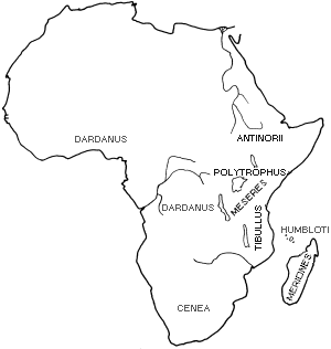
p and q, the frequencies of the model (as assessed by the collector) and mimic, can be taken from Ford (1936) for the races meseres and polytrophus, where he cites data from random collections by van Someren in 1923 and Wiggins some time before 1910. These are shown in Table 7-7.

Of course, the non-mimetic forms (such as the andromorphic trimeni) will have no models at all, so will gain no protection from predators.

These parameters (the relative proportions of model and mimic, and the 'memory' parameter affected by the relative palatabilities of model and mimic) will be varied and the results discussed in the 'mathematical model' section of this chapter which follows.

The mathematical model

Introduction

The factors listed above were all incorporated into a model of the population in the form of a computer program written in C (see Appendix 6 for a program listing). The model simulated the change in morph proportions through successive generations under the conditions imposed. Each parameter which has been assessed above was entered into the model, leaving the unknown value of Huheey's 'memory parameter' and the rate of predation to be varied.

Method

The first population to be modelled was the race polytrophus, with the values of the ratio of model to mimic as reported in Ford (1936) and shown in Table 7-7. Ford gave values for only three morphs (although trophonius is reported as being present in the race - see Appendix 1), two mimetic (although he reported no models of hippocoonides, so the ratio of model:mimic was taken to be 5:53) and one he reports to be non mimetic (he calls it salaami, although it no doubt equates to the form poultoni as described in Appendix 1 as present in race polytrophus). The proportions reported for these three morphs in Table 7-7 were therefore entered as the starting proportions, and the values of the memory and predation pressure parameters varied in an attempt to find a stable balance of the morphs.

The second population to be modelled was that from Pemba, Tanzania - studied by Cook et al. (1994). Unfortunately for this population the ratio of the models to the mimics was not assessed accurately, although the model of the rarer mimic (trophonius) was reported to be rare also (pers. comm.), and so the ratios were set to 1:1 for each of the two mimetic morphs (the non mimetic morph trimeni had no model, of course). Once the optimum parameters for stability had been found, then the ability of the different morphs to invade a monomorphic or dimorphic starting population were investigated.

Results

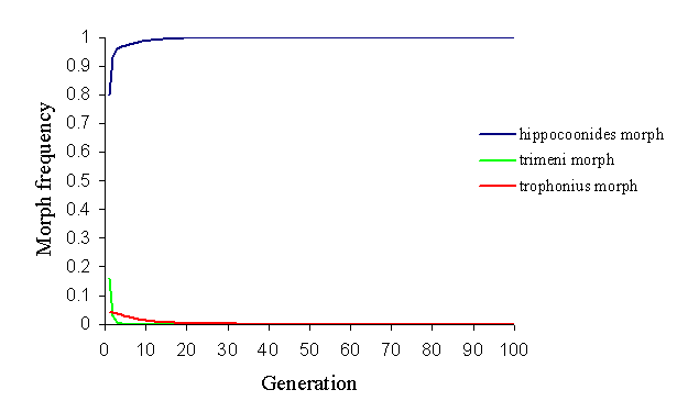
In the polytrophus race, it is clear from looking at the starting proportions that salaami is never going to be maintained in the population under the conditions imposed by the model. The mate choice favours the most common morphs, and the predator pressure favours the mimetic morphs. Therefore a non-mimetic, rare morph is always going to be excluded from the population whatever the variable parameters are set to. This is shown by the model in Figure 7-3.

Figure 7-3 Mathematical model of the polytrophus population showing that the rare, non-mimetic morph (salaami) cannot be maintained in the population (parameters: probability second mating= 0.59, probability choosing same morph twice = 0.75, probability encounter predator before mating = 0.95, memory of predator = 40, abundance of models and mimics as in Table 7-7).

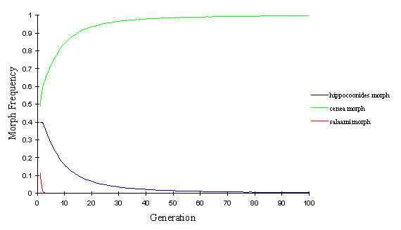
The hippocoonides morph declines as it has much less protection from predators then cenea, and also starts at a lower frequency, and thus is slightly disadvantaged with respect to mate choice.

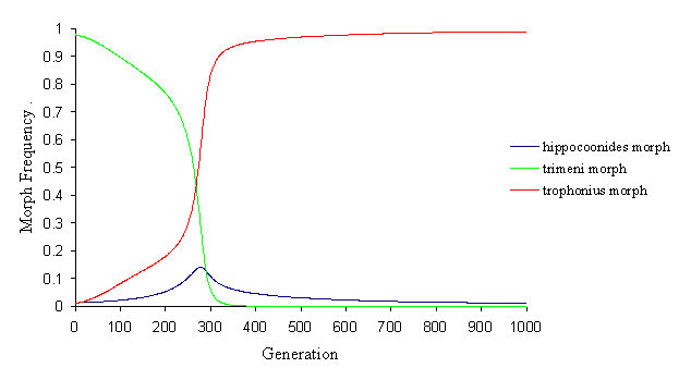
In the race meseres, Ford (1936) reported no non-mimetic morphs. However, using the figures from Table 7-7 ( and removing niobe from the population, since the model is only written to simulate three morphs in a population) it is still not possible to balance the morphs in the population (see Figure 7-4). This is because the only variables are the encounter rate and memory of the predators, and this will only alter the amount of advantage in natural selection of the most protected morph. Since the sexual selection pressure is so strong, it is impossible to counter the effect on the most common morph, even though it is the least protected in terms of the initial ratio of model to mimic, and its increasing frequency decreases the ratio of model to mimic.

Figure 7-4 Mathematical model of the meseres population showing that the rare morphs cannot be balanced in the population (parameters: probability second mating= 0.59, probability choosing same morph twice = 0.75, probability encounter predator before mating = 0.95, memory of predator = 40, abundance of models and mimics as in Table 7-7).

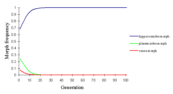
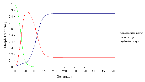
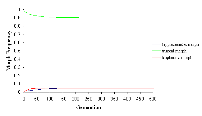
In the Pemba population, the relatively rare andromorph will again be at a disadvantage both in natural and sexual selection according to this model, and hence it would be expected to be eliminated from the population. With the strong sexual selection advantage conferred upon the most common morph (in this case, hippocoonides), it is also not possible to keep the rare trophonius in the population, even by reducing the probability of choosing the same morph twice to 0.5 (see Figure 7-5).

Figure 7-5 Mathematical model of the Pemba population, showing that trimeni and trophonius can never be maintained under this model (parameters: probability second mating = 0.59, probability choosing same morph twice = 0.5, probability encounter predator before mating = 0.9, memory of predator = 1000, initial frequencies of each morph as in Appendix 5, initial ratio model:mimic for hippocoonides = 1, for trophonius = 1000).

Even by decreasing the advantages of hippocoonides by increasing massively the protection of trophonius (by increasing the ratio of models to mimics) and the memory of the predators (to strengthen the protection to trophonius), hippocoonides is too common at the outset to be maintained.

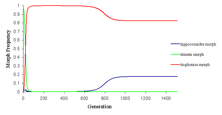
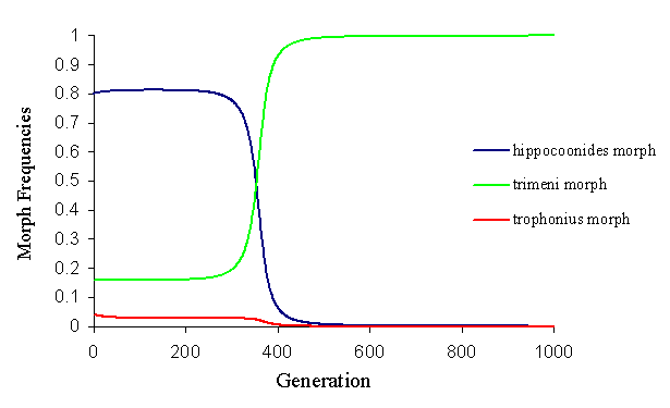
It is possible to investigate the evolution of the different morphs by running the simulation with a monomorphic starting population (and a tiny proportion of new mutant morphs). The initial starting population was first taken to be monomorphic andromorphs. With different parameters, the final outcome of the population can be very different. In some cases, one or other of the mimetic morphs goes to fixation in the population (although the dynamics of this can be very interesting, as in Figure 7-6).

Figure 7-6 Mathematical model of invasion of hippocoonides and trophonius morphs in a monomorphic population of trimeni showing one of the mimetic morphs going to fixation (parameters: probability second mating = 0.59, probability choosing same morph twice = 0.5, probability encounter predator before mating = 0.3, memory of predator = 11, initial frequency trimeni = 0.98, frequencies of other morphs = 0.01, initial ratio model:mimic for hippocoonides = 4, for trophonius = 2.5).

Here, the andromorphs immediately start to decline, due to predator pressure, and their place is taken by both trophonius and hipppocoonides. The dominant trophonius, however, does slightly better than hippocoonides initially, and as the decline of the andromorphs starts to accelerate (as they lose the sexual selection advantage), trophonius starts to increase rapidly, and hippocoonides again goes into decline as trophonius has an advantage in both natural and sexual selection.

Another alternative is that the two invasive mimetic morphs come to balance, whilst eliminating the non-mimetic andromorph (see Figure 7-7 and Figure 7-8).

Figure 7-7 Mathematical model of invasion of hippocoonides and trophonius morphs in a monomorphic population of trimeni showing hippocoonides and trophonius coming to balance (parameters: probability second mating = 0.59, probability choosing same morph twice = 0.5, probability encounter predator before mating = 0.5, memory of predator = 11, initial frequency trimeni = 0.98, frequencies of other morphs = 0.01, initial ratio model:mimic for hippocoonides = 4, for trophonius = 2.2).

Figure 7-8 Mathematical model of invasion of hippocoonides and trophonius morphs in a monomorphic population of trimeni showing hippocoonides and trophonius coming to balance (parameters: probability second mating = 0.59, probability choosing same morph twice = 0.5, probability encounter predator before mating = 0.5, memory of predator = 11, initial frequency trimeni = 0.98, frequencies of other morphs = 0.01, initial ratio model:mimic for hippocoonides = 4, for trophonius = 6).

This alteration of the fortunes of each mimetic morphs is achieved simply by slight increases or decreases in the initial ratio of model to mimic (which, of course, varies as the morph frequencies vary), to which the mathematical model is very sensitive, and this demonstrates why the morph balance changes so rapidly across areas where the balance of the different models changes.

By altering the parameters, however, it is possible to balance the factors ending in a balanced polymorphism of all three morphs, with varying proportions of each morph (see Figure 7-9 and Figure 7-10).

Figure 7-9 Mathematical model of the invasion of hippocoonides and trophonius morphs into an andromorphic population resulting in a balanced situation (parameters: probability second mating = 0.59, probability choosing same morph twice = 0.5, probability encounter predator before mating = 0.5, memory of predator = 3, initial frequency trimeni = 0.98, frequencies of other morphs = 0.01, initial ratio model:mimic for hippocoonides = 1, for trophonius = 1).

Figure 7-10 Mathematical model of the invasion of hippocoonides and trophonius morphs into an andromorphic population resulting in a different polymorphism (parameters: probability second mating = 0.59, probability choosing same morph twice = 0.5, probability encounter predator before mating = 0.5, memory of predator = 5, initial frequency trimeni = 0.98, frequencies of other morphs = 0.01, initial ratio model:mimic for hippocoonides = 1, for trophonius = 1).

This change in the population structure was achieved by altering the memory of the predator (which is affected not only by the predators, but also by the relative distastefulness of the models and mimics). It shows how andromorphs may be maintained in a balanced polymorphism as long as they remain above a certain threshold level. If they fall below about 50% in the population, they lose their sexual selection advantage, and are rapidly eliminated from the population.

If the population does not include andromorphs there is, of course, no way in which they can invade, and even if the starting population is dimorphic, with a high proportion of andromorphs to mimetic morphs, the added advantage of the mimicry leads to the andromorphs becoming rapidly extinct (see Figure 7-11). Therefore in the current model, the only way in which andromorphs can be maintained in the population is for them to be the ancestral, monomorphic condition and for them to remain at a relatively high proportion in the population when mimetic morphs invade.

Figure 7-11 Mathematical model showing the demise of the andromorphs in an initially dimorphic population with a high proportion of andromorphs (parameters: probability second mating = 0.59, probability choosing same morph twice = 0.5, probability encounter predator before mating = 0.5, memory of predator = 5, initial frequency trimeni = 0.80, frequency hippocoonides = 0.19, freqency trophonius = 0.01, ratio model:mimic for hippocoonides = 1, for trophonius = 1).

Cook et al. (1994) and Vane Wright (1984) suggest that the andromorphs may have an advantage in sexual selection, although Vane Wright's 'pseudosexual selection' hypothesis maintains that this advantage is through increased matings due to males approaching andromorphs as if they were males (for aggressive encounters), whilst Cook et al. suggest that the andromorphs are approached less often, and that this lack of sexual harrassment provides the andromorphs with an advantage. Although the naïve males in behavioural experiments in Chapter 5 appeared to mate at random, no andromorphs were available to test the either hypothesis, and so a preference or avoidance of andromorphs cannot be ruled out in this species.

It is possible to alter the mathematical model to alter the probability of a male mating with each morph on his first mating. This allows the pseudosexual selection hypothesis to be investigated. Cook et al.'s sexual harrassment hypothesis effectively amounts to the same thing - in reality the andromorphs are not being mated more frequently (as the model suggests), but the result of them leaving more offspring is the same.

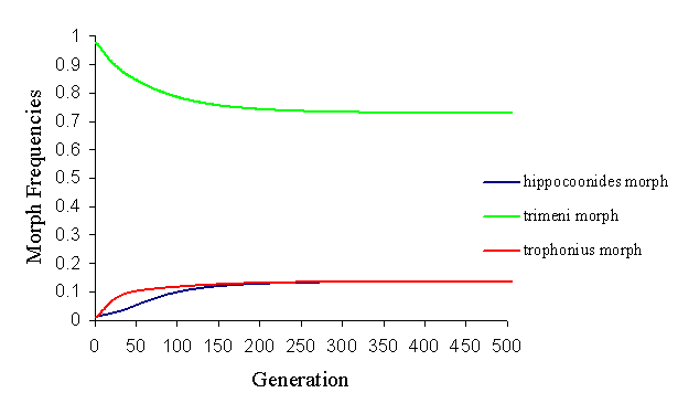
If Cook et al.'s frequencies of approaches to each morph are used as the frequencies of initial matings (although the inverse is taken, as they assume increased approach to be detrimental), it is not possible to achieve a balanced polymorphism of all three morphs (by altering the predation parameters), but it is easy to balance hippocoonides and trophonius (see Figure 7-12).

Figure 7-12 Mathematical model using initial mating frequencies from Cook et al. (1994), showing that andromorphs still cannot be maintained (parameters: probability second mating = 0.59, probability choosing same morph twice = 0.5, probability encounter predator before mating = 0.5, memory of predator = 5, initial frequencies of morphs, and initial mating frequencies as in Appendix 5, ratio model:mimic for hippocoonides = 1, for trophonius = 1).

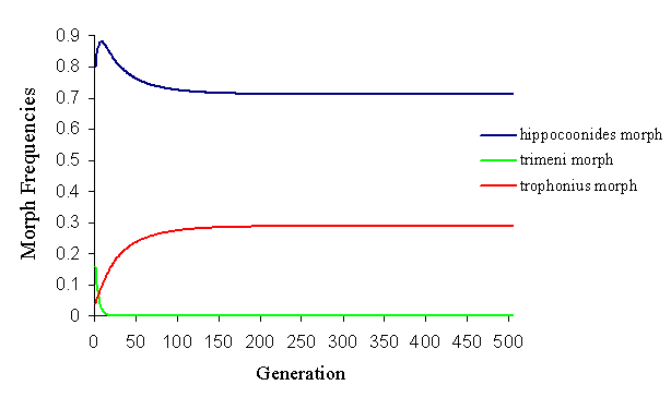
By altering these initial mating frequencies, it is almost possible to achieve the balanced polymorphism seen in the wild population. However, due to the strong frequency-dependent mate choice (and the frequency-dependent predator pressure), this balance is on a knife edge, and any slight perturbation causes it to break down very rapidly (see Figure 7-13).

Figure 7-13 Mathematical model demonstrating a knife-edge polymorphic balance, achieved by altering initial mating frequencies and predator parameters (parameters: probability second mating = 0.59, probability choosing same morph twice = 0.5, probability encounter predator before mating = 0.5, memory of predator = 5, initial frequencies of morphs as in Appendix 5, initial mating frequency for hippocoonides = 0.45, for trimeni = 1, for trophonius = 0.722, ratio model:mimic for hippocoonides = 1.8587, for trophonius = 1.8587).

Discussion

The model clearly illustrates that under the conditions imposed by the factors discussed earlier in the chapter, the low proportions of non-mimetic morphs reported from some populations of Papilio dardanus cannot be stable. Therefore these populations are either not balanced, and are undergoing the loss of non-mimetic morphs, or there are other factors acting which have not been taken into account. The first of these explanations seems unlikely as, although the population balance may well shift through time, the model shows a very rapid extinction of non-mimetic forms, and the forms reported over 50 years ago by Ford (1936) and others are still present in the populations, several hundred generations later.

It seems, therefore, that pressures other than those considered in this thesis may be acting. In the mate choice experiments it was not possible to obtain enough non-mimetic morphs to carry out choice tests using them. This is unfortunate, as it has therefore not been possible to test the 'pseudosexual selection' hypothesis (Vane Wright, 1984) in which andromorphic females are approached more often by males as they are mistaken for males and thus approached aggressively or the opposite view put forward by Cook et al. (1994), who suggested that excess male attention may be a handicap to females. Both theories suggest an advantage to andromorphs through a varying initial approach rate, which has been shown in this model to be unlikely to hold the polymorphism in a stable balance if there is a learning effect in the male mate choice due to the magnifying effect this has on small perturbations in the proportions of the morphs. Behavioural observations (see Chapter 5) suggest that males do approach other males more often than females, running counter to the observations of Cook et al. (1994) who found trimeni females to be approached less often than hippocoonides females by wild males.

By altering the model to take into account varying frequencies of initial matings for each morph it is possible to obtain a balanced polymorphism as seen in the wild populations, but the strong frequency-dependent selection pressures in both natural and sexual selection make this balance very easily perturbed, and therefore the wild populations might be expected to show morph fluctuations. Since no regular morph frequency assessments have been reported for the species, it is not possible to say whether or not this does actually occur. However, the model does illustrate how sensitive the morph frequencies are to changes in the ratio of model to mimic, and this is seen in wild populations where morph frequencies change to match those of the models (Ford, 1936).

The model shows how it is possible under the conditions imposed for a monomorphic non-mimetic population to be invaded by mimetic morphs, but for the non-mimetic morphs still to be maintained (as long as they do not fall below a certain threshold of frequency). This may be similar to the conditions seen in race antinorii, where the andromorphs are very frequent in the population, and the mimetic morphs are kept relatively rare. It is, however, much more difficult for andromorphs to invade a mimetic population - without the added advantage of differing rates of initial matings it is impossible, and the advantage which would need to be conferred to allow it would be very great indeed. It therefore seems more likely, on the basis of this population model, that the andromorphic females are ancestral to the mimetic morphs.

Conclusions

This thesis has examined the ways in which butterflies receive and perceive visual signals. In the case of Argynnis paphia, the males appear to show a preference for orange when choosing mates and flowers which is not related to their signal reception. This implies that the preference is due to their perception of the colour - either they have evolved a preference which allows them to recognise the orange females as mates which also has the effect of causing them to prefer orange flowers, or they have an unselected 'hidden preference', which might even have been exploited subsequently by the orange female morph. It has not been possible to distinguish between these two possibilities, although mate choice work carried out in a population which was dominated by the green female morph may be illuminating. It would also be necessary to carry out experiments to determine whether or not the males are learning the preference for orange females.

The work on Papilio dardanus has brought to light several behaviour patterns which have not been reported before. Firstly, the butterflies have been shown to have a preference for blue flowers over red and yellow (a pattern which is seen in other Papilionids: Ilse, 1928; Ilse & Vaidya, 1956; Swihart, 1970). The lack of interest in red flowers can be explained by their lack of spectral sensitivity in this area of the spectrum, but this does not explain their preference for blue over yellow. Further experiments suggested that colour may not be the most important factor for the butterflies as their preference could change dramatically to red if the flowers were left unpainted. What caused this switch in behaviour has still to be discovered. It was also shown that individual butterflies tended to be 90% constant to a particular colour when they were rewarded for visiting that colour (but some data suggested that they tended to try other colours if their first choice did not provide food). For the first time it was demonstrated that the presence of other butterflies feeding could influence the behaviour of individuals, causing them to choose flowers which were spatially close to that on which another butterfly was feeding, regardless of its colour.

It was not possible to test whether or not male Papilio dardanus would show a preference for blue female morphs, as they could not be made to react to models or altered females. However, naïve males appeared to mate at random when first encountering females, not showing any colour preferences at all. When mated males were subsequently given the same choice of females, however, they tended to prefer females of the morph with which they had already successfully mated. This apparent colour constancy and rapid learning is similar to that seen in the flower choice experiments, but the initial preference is lacking.

The model of random mating followed by rapid learning from a first mating would, in general, explain the results of Cook et al. (1994) who found that male Papilio dardanus showed a significant preference for the most common morph. The actual data acquired by Cook et al. cannot be explained simply by such a model of behaviour, but discrepancies could be due to the pair-wise presentation methods employed and the self-selecting nature of the experimental butterfly group.

It has not been possible to assess accurately the palatability of Papilio dardanus relative to its distasteful models, although starlings appeared to find the species entirely palatable (see Chapter 6). An indirect measure of the palatability, the morphology of the butterflies (also assessed in Chapter 6), suggests that Papilio dardanus is indeed a Batesian mimic, as the centre of mass of the males is in the position expected for palatable species. The females, however, were shown to have a centre of mass further from the wingbase than both males and both sexes of Danaus chrysippus, which would cause them to be more prone to capture by birds than males (Srygley & Dudley, 1993), and it is possible that this has been a factor causing female-limited mimicry in this species. This was not true of Danaus chrysippus, where males and females showed similar positions of the centre of mass. In addition, Srygley (1994) found that mimetic species tended to have centres of mass placed further back from the wingbase than non-mimetic species. Taken together, this evidence suggests that the position of the centre of mass, and its effect on the agility of a butterfly in flight, may be a factor affecting the evolution of mimicry in a species, or (where the egg load of the females causes their centre of mass to be placed further back) in only the females of a species.

When this mate choice and palatability information is assessed by means of creating a mathematical model of the balance of the morphs in a population, it can be seen that for the model to explain the current morph balances in different populations an initial mating advantage for non-mimetic morphs has to be introduced. This could be investigated by continuing mate choice experiments similar to those in Chapter 5, but using andromorphic and non-mimetic females as well as those already studied. It appears likely that andromorphic females are gaining an advantage in sexual selection, although there are two opposing hypotheses to explain this (Cook et al., 1994 and Vane Wright, 1984). From behavioural observations in the flight cage (see Chapter 5) it appears likely that the males would approach andromorphic females more often than mimetic females, in accordance with the pseudosexual selection theory (Vane Wright, 1984), although this has yet to be tested. Some of the morphs described as non-mimetic which are not andromorphic may well in fact be mimetic, at least to some degree, of unidentified butterflies, which would give them some protection from predators, and the presence of a pyrazine odour is likely to reinforce this protection (Rowe & Guilford, 1996).

The model also suggests that the andromorphic females are most likely to be ancestral to the mimetic females, as the frequency-dependent sexual selection makes it very difficult for them to invade a mimetic population. A molecular genetic approach, however, is likely to shed further light on the evolution of the species and its morphs.

Acknowledgements

I am very grateful to John Alden for help with C programming and to Yan Wong for help with modelling techniques, and to both for help in creating the Papilio dardanus population genetics Website. I would also like to thank Nigel Venters for discussions about wild populations of Papilio dardanus.

References

Avery, M.L. 1985. Applications of mimicry theory to bird damage control. J. Wildl. Mgmt. 49, 116-121.

Brower, J.V.Z. 1960. Experimental studies of mimicry. Part IV. The reactions of starlings to different proportions of models and mimics. Am. Nat. 94, 271-282.

Burns, J.M. 1968. Mating frequency in natural populations of skippers and butterflies as determined by spermatophore counts. Proc. Nat. Acad. Sci. 61, 852-859.

Cook, S.E., Vernon, J.G., Bateson, M., Guilford, T. 1994. Mate choice in the polymorphic African swallowtail butterfly, Papilio dardanus: male-like females may avoid sexual harassment. Anim. Behav. 47, 389-397.

Drummond, B.A. 1984. Multiple mating and sperm competition in the Lepidoptera. In Sperm competition and the evolution of animal mating systems (ed. Smith, R.L.). Academic Press, London. P291-370.

Ford, E.B. 1936. The genetics of Papilio dardanus Brown (Lep.) Trans. R. Ent. Soc. London 85, 435-465.

Huheey, J.E. 1980. Studies in warning coloration and mimicry. VIII. Further evidence for a frequency-dependent model of predation. J. Herpetol. 14, 223-230.

Huheey, J.E. 1988. Mathematical models of mimicry. Am. Nat. 131, S22-S41.

Ilse, D. 1928. Über den Farbensinn der Tagfalter. Z. f. vergl. Physiologie Bd. 8, 658-692.

Ilse, D. & Vaidya, V.G. 1956. Spontaneous feeding response to colours in Papilio demoleus L.. Proc. Indian Acad. Sci., Sect. B 43, 23-31.

Lederhouse, R.C. 1981. The effect of male mating frequency on egg fertility in the black swallowtail, Papilio polyxenes asterius (Papilionidae). J. Lepid. Soc. 35, 266-277.

Makielski, S.K. 1972. Polymorphism in Papilio glaucus L. (Papilionidae): maintenance of the female ancestral form. J. Lepid. Soc. 26, 109-111.

Pliske, T.E. 1972. Sexual selection and dimorphism in female tiger swallowtails, Papilio glaucus L. (Lepidoptera: Papilionidae): A reappraisal. Ann. Entomol. Soc. Am. 65, 1267-1270.

Pliske, T.E. 1973. Factors determining mating frequencies in some New World butterflies and skippers. Ann. Entomol. Soc. Am. 66, 146-169.

Rothschild, M., Von Euw, J., Reichstein, T., Smith, D.A.S., & Pierre, J. 1975. Cardenolide storage in Danaus chrysippus with additional notes on D. plexippus. Proc. R. Soc. B 190, 1-31.

Rowe, C. & Guilford, T. 1996. Hidden colour aversions in domestic chicks triggered by pyrazine odours of insect warning displays. Nature 383, 520-522.

Shields, O. 1967. Hilltopping: an ecological study of summit congregation behaviour of butterflies on a southern California hill. J. Res. Lepid. 6, 69-178.

Sims, S.R. 1979. Aspects of mating frequency and reproductive maturity in Papilio zelicaon. Am. Midl. Nat. 102, 36-50.

Srygley, R.B. 1994. Locomotor mimicry in butterflies? The associations of positions of centres of mass among groups of mimetic, profitable prey. Phil. Trans. R. Soc. Lond. B 343, 145-155.

Srygley, R.B. & Dudley, R. 1993. Correlations of the position of center of body mass with butterfly escape tactics. J. Exp. Biol. 174, 155-166.

Svärd, L. & Wicklund, C. 1986. Different ejaculate delivery strategies in first versus subsequent matings in the swallowtail butterfly, Papilio machaon L. Behav. Ecol. Sociobiol. 18, 325-330.

Swihart, S.L. 1970. The neural basis of colour vision in the butterfly Papilio troilus. J. Insect Physiol. 16, 1623-1636.

Turner, J.R.G. & Speed, M.P. 1996. Learning and memory in mimicry. I. Simulations of laboratory experiments. Phil. Trans. R. Soc. Lond. B 351, 1157-1170.

Vane Wright, R.I. 1984. The role of pseudosexual selection in the evolution of butterfly colour patterns. In The Biology of Butterflies (ed. Vane Wright, R.I. & Ackery, P.R.) Princeton, USA.